This article describes how I built a service to provide map tiles in a vector-based format using Open Street Map data.
Background
About 4 months ago I joined The Tap Lab, a currently 10-person mobile gaming startup in Cambridge. I came on board just in time for the launch of their first major title, an empire building game for iOS called Tiny Tycoons. The game is played on what is essentially a stylized Google Maps, with an isometric view of your avatar moving amongst labeled streets and sprites representing real local businesses at which you can perform jobs to earn coins. Once you have earned enough coins you can purchase these businesses, which then become sources of revenue themselves. The game world is shared by all players, so only one person can own, say, the Starbucks in Davis Square. Players essentially compete to become virtual real-estate tycoons by buying up properties all over the world.

All information about local businesses is pulled from Foursquare; for example, the number of check-ins is used to calculate a property’s value in the game. Map data such as roads, bodies of water, and cities/towns are pulled from a service called Cloudmade. This is done via the traditional tile format, where the world is divided into some number of tiles depending on the zoom level and each is referenced by an x/y coordinate. The API is passed x/y/zoom parameters and returns map data for the given tile. Most major services, such as Google maps and Cloudmade, provide this data in the form of an image. Cloudmade also has an experimental service that provides this data in vector form via SVG, which is what we use for our game. While we can fall back to image tiles, vector tiles allow us to better place the local business sprites so they do not appear in the middle of roads, as the latitude and longitude coordinates from Foursquare are not precise enough to accomplish this on their own.
Unfortunately, Cloudmade has decided to discontinue this service and focus on their presumably more popular image tile API. We were first informed of this sometime this past July when the service was switched off abruptly; after a good amount of panic and complaining, they switched it back on but told us it would be officially retired on August 1st. We quickly implemented the image tile fallback in the event this happened again, but it was slower and looked pretty awful, with property sprites being placed haphazardly. I was tasked with finding a replacement, preferably before the August 1st shutdown date. I should note here that even now, well into August, the service is still up.
I had almost no background on mapping systems going into this project and I am still nowhere close to an expert on the subject. I had assumed that vector-based map data was the default and that we could just switch to another provider; either Google/Apple Maps or OpenStreetMap if the formers’ Terms of Service were too onerous or they were too expensive. I quickly discovered that the major services only offered image tiles and that vector tiles were in fact only just beginning to become a thing (hence Cloudmade’s “experimental” API) due to their potential for custom styling of geographic features and metadata. Google and co. likely have proprietary vector data underlying their image tiles, but at the moment they aren’t sharing.
OpenStreetMap
I wondered if OpenStreetMap, which I knew nothing about and assumed was an open-source clone of Google Maps, had similar underlying vector data that was open and accessible. I was brought to a page on the wiki detailing the current state of vector tiles running on top of OSM data. As I discovered and as you may already know, OSM is not so much a full-stack service as it is a raw data source of geographical elements that the community submits and maintains. Services are then built on top of this data. Some, such as the official API, just provide access to the raw XML data, mostly for the purposes of editing and submitting. Others, including some of the major map services if I’m not mistaken, take that data and turn it into the image tiles we are familiar with. The wiki pointed to one or two research projects that combined various layers of software such as Mapnik on top of the data to create vector tiles. There was the possibility of replicating these stacks, but they were quite complex, cutting edge solutions created by experts in the mapping community and doing so would be no small task.
One of the articles linked in the wiki mentioned that you could theoretically bootstrap a rough approximation of a vector tile service by using the bounding box query of the standard OSM API, querying over the same area as the desired tile and transforming the returned XML into vector data. This seemed like a good place to start, though it sounded a little hackish and rough around the edges. I also found that several other providers offer the basic OSM API, as the one run by the community is for contributing data and is not for production use. Some also offered the OSM XAPI, which contained additional parameters for querying elements. Among these providers was MapQuest, which offers a beta service exposing the OSM XAPI for free. This was a relief, as the alternative is downloading the half-terabyte (and growing) OSM dataset, importing it into a database with geo-spatial support, setting up and configuring the necessary software and hosting the API oneself.
The bounding box query allows you to specify a left and right latitude and a bottom and top longitude and returns all geo-data contained within that box in an XML format. This data consists of 3 different types of elements: nodes, which represent particular points and places; ways, which are made up of references to nodes and represent either linear elements like roads, rivers and coastlines or closed polygons like lakes and other defined areas; and relations, which consist of collections of the other elements that aren’t important for our purposes. Each of these elements can have “tag” sub-elements containing key-value metadata pairs, such as the name of a road and how many lanes it has. Many of these tags are standardized by the OSM community and can be queried in a (very) basic fashion by the XAPI, in addition to being able to filter on the types of top-level elements themselves. Lastly, each node element has an attached lat/lon coordinate.
Example query:
/xapi/api/0.6/way[highway=primary|secondary|residential][bbox=-77.0265,38.8924,-77.0222,38.8943]
This queries for all way elements that are tagged as highways (standard tag for roads of any type) with either of 3 different values denoting road type, all within a small area in Washingon DC. The abridged XML returned looks something like this:
<?xml version='1.0' encoding='UTF-8'?>
  <osm version="0.6" generator="Osmosis SNAPSHOT-r26564">
    <bound box="38.89243,-77.02656,38.89431,-77.02227" origin="Osmosis SNAPSHOT-r26564"/>
    <node id="49748733" version="4" timestamp="2009-10-08T22:25:23Z" uid="147510" user="woodpeck_fixbot" changeset="2788109" lat="38.892082" lon="-77.02599" />
    ...

    <way id="6061126" version="4" timestamp="2011-09-27T19:27:51Z" uid="207745" user="NE2" changeset="9413560">
      <nd ref="49748733"/>
      <nd ref="49827578"/>
      <tag k="highway" v="residential"/>
      <tag k="name" v="10th St NW"/>
      ...
    </way>
    ...
</xml>
Compare this with a query to Cloudmade’s vector tile server and it’s corresponding response in SVG:
http://alpha.vectors.cloudmade.com/API_KEY/STYLE_ID/256/18/79299/96970.svgz
Note that in this query, 256 represents the width and height in pixels of the resulting image if the SVG were to be rendered. The zoom level is specified at 18; zoom levels for most map services tend to run from 0-20, with 0 being zoomed out all the way so as to see the entire Earth, and 20 being whatever the maximum magnification allowed by the mapping service. Our game uses levels 15-18, as anything lower is impractical for gameplay. The x and y coordinates of the tile are specified as 79,299 and 96,970 respectively. The abridged SVG output is below:
<?xml version='1.0' encoding='UTF-8'?>
<svg xmlns="http://www.w3.org/2000/svg" xmlns:cm="http://cloudmade.com/" width="256" height="256">
  <rect width="100%" height="100%" fill="#98bcda" opacity="1"/>
  <g transform="scale(1.67458095912)">
    <g transform="translate(7914748, 5213311)" flood-opacity="0.1" flood-color="grey">
      <path d="M -7914613.65 -5213184.5 l -42.24 57.69 -42.04 54.47 -22.15 28.75 -22.75 29.53 -43.96 55.42 -67.83 87.9 -54.47 70.71 -16.17 18.27" fill="none" stroke="#686868" stroke-width="5.27296094697px">
        <cm:z_order>6</cm:z_order>
        <cm:name>Brookline Avenue</cm:name>
        <cm:cm_id>43100850</cm:cm_id>
        <cm:timestamp>2011-01-03 14:28:28+00:00</cm:timestamp>
        <cm:width>19.5</cm:width>
        <cm:highway>secondary</cm:highway>
      </path>
      ...
    </g>
  </g>
</svg>
The SVG essentially consists of a collection of path objects, each representing some geo element composed of a set of points forming either a line or a closed polygon. This representation is all that is needed for the elements used in the game: roads, rivers, coastline, and bodies of water. The “d” attribute of each path denotes the set of points. The letter “M” in the string means “move to this absolute point”, and is followed by an x and y coordinate. “l” (lowercase L) means “draw a line to this position, which is specified by a set of coordinate pairs that are relative to each previous point, starting with the aforementioned absolute point”. If the “d” attribute ends with a “z”, that means the path is to be closed into a polygon. The path also contains styling information specifying how it should be drawn, and contains child elements denoting metadata associated with the path such as its name. For more information, see the SVG specification.
Additionally, there are a couple of transform tags present at the beginning of the file. You may have also noticed that the coordinates in the paths are way outside the bounds of a 256×256 image and are wondering how they are rendered. As it turns out, these two things are related. Cloudmade’s coordinates are in a global pixel space based on a Mercator projection, with 1px=1m and a width and height equal to the Earth’s circumference with an origin in the center. These global coordinates are converted into the local image coordinate space, which has a height and width of 256px and the origin in the top left, by applying a series of transformations. The first is a translation, where an x and y value are added to the absolute coordinates only (the “M” coords) to make them relative to the local origin. Then, you multiply all coordinates (absolute and relative) by the scale factor.
Depending on your needs, it is not strictly necessary to specify the coordinates like this. If there’s no need for the consuming application to know the absolute global position of these elements, they can simply be specified in local coordinate space without the transforms. What is necessary for most applications however is a tiling system, as it is the industry standard way for dealing with map data in a scalable fashion. I’ll go into more detail about this shortly.
As you can see, the OSM XML and the desired SVG data formats are fundamentally the same; they both contain a set of geo elements with their attached metadata, specified as a series of coordinates. They are really just a simple XML transformation away from each other. The notable exception to this is that the OSM query and results are in latitude and longitude, whereas the Cloudmade query and results are in desired tile and local coordinate space, respectively. How do we get from one to the other?
Coordinate Transformation
A tiling system divides the globe up into equally-sized square tiles, referenced by x/y coordinates. The number and size of these tiles depends on the zoom level, or how close the observer is to the Earth. As mentioned before, this is usually a number Z between 0 and 20, where the world is divided into 2^Z x 2^Z tiles. So if we are at zoom level 0, the entire world is contained within 2^0 = 1 tile. If we are at zoom level 5, the world is divided into 2^5 = 64×64 tiles, and so on. Of course, this only works if the world is projected onto a rectangular plane. The projection commonly used in the mapping community seems to be the Spherical Mercator projection, and there are standard equations used to convert latitude/longitude coordinates into x/y coordinates and back again. I am not going to dig into them here, as I don’t fully understand them myself and there are a variety of different implementations of the same equation. Cloudmade provides a helpful page in their docs with their implementation (scroll to the bottom):
Convert lat/lon to tile coords:

n = 2 ^ zoom
xtile = ((lon_deg + 180) / 360) * n
ytile = (1 - (ln(tan(lat_rad) + sec(lat_rad)) / Pi)) / 2 * n

Note: ln stands for natural logarithm, sec = 1/cos
Round down xtile and ytile to get the integer tile numbers.

If you need to go the other way:

n = 2 ^ zoom
lon_deg = xtile / n * 360.0 - 180.0
lat_rad = arctan(sinh( Pi * (1 - 2 * ytile / n)))
lat_deg = lat_rad * 180.0 / Pi
The second set of equations allows you to get the lat/lon coords of the top-left corner of a given tile, which is also the top-left corner of the equivalent bounding box. The bottom-right corner of the box is simply the top-left corner of the tile one down and one over to the right (the origin of the world in tile-space is in the top left corner, so the next tile is at x+1, y+1). Since the bounding box query requires you specify the bottom-left and top-right coordinates, you’ll have to swap these around, but otherwise that is all you need to generate an OSM bbox query from a set of x/y/zoom tile coordinates.
It is similarly straightforward to convert the lat/lon coordinates for the various geo objects returned by the query into pixel coordinates for a 256×256 image (or whatever size is desired). Recall that we now have the top-left corner, in latitude and longitude, of the bounding box/tile these geo elements lie within. We also have the width and height of the bounding box (right minus left, top minus bottom; it is important to remember that longitude corresponds to x, and latitude to y) in lat/lon degrees as well. If we subtract the left coordinate of the box from the longitude of the point, and the latitude from the top coordinate (remember, the world origin is in the middle, whereas the local image origin is in the top-left), we get the point’s position in lat/lon relative to the top-left corner of the box. If we then divide these coordinates by the height and width respectively, we get normalized coordinates between 0 and 1 within the bounding box, which we can then multiple by our image size (256) to get the local image coordinates. To illustrate more clearly:
width = bbox.right - bbox.left
height = bbox.top - bbox.bottom

x = (point.longitude - bbox.left) / width * 256
y = (bbox.top - point.latitude) / height * 256
That is, of course, for the first absolute point in each path, the “M” point. Each subsequent point has it’s coordinates calculated relative to the previous point’s lat/lon rather than the bounding box’s, in order to get the relative “l” coordinates.
Implementation and Styling
I’m not going to go into the implementation details of querying the OSM endpoint, parsing the XML, building paths by transforming the coordinates of the nodes/ways, and outputting the result to SVG; all of that should be fairly straightforward, if somewhat laborious, with the information I’ve provided here. Determining whether to close each path to form a polygon and what color to set the fill or stroke to depends on what type of geo element it is, which can be gleaned from a <way> element’s tags in the OSM XML. As mentioned previously, all roads have a “highway” tag with a variety of standard values that can be looked up on the OSM wiki and can be used to determine the color and, along with a function of zoom level, the width based on stylistic preferences. Bodies of water such as lakes are tagged with “natural=water”; rivers are tagged with “waterway=river”, but if you want more than just a line of indeterminate width you can look for “waterway=riverbank”, which will give you a closed polygon with edges representing the actual banks of the river. Coastlines are tagged with “natural=coastline” and are a special, extremely difficult case, which is why I’m going to cover them in detail next.
Coastlines
Coastlines are a unique challenge when attempting to render OSM data for several reasons. The primary obstacle is that while coastlines are returned from the bbox query as path segments similar to roads and rivers, they in fact represent portions of extremely large polygons (the Earth’s oceans). It is obviously impractical for the OSM API to return the entire polygons, but it will also not create a smaller polygon out of the path and the bbox for you; you must do this yourself, and it is not a trivial task. In fact, the vast majority of the time I spent on this project was dedicated to getting coastlines to render properly, which is why I’m going to dedicate a large portion of this article to it.
Additional issues that further complicate this task include the fact that the coastlines returned by the API maybe be in several different pieces. You can generally assume that these pieces are connected by shared start/end points, as the OSM community periodically runs a job on the data to make sure the coastlines are smooth. The API will return any segments of coastline that pass through your bounding box; you should also be aware though that it will often return pieces that don’t as well (though they will still be close by), and that you can’t really depend on which of these out-of-bounds pieces it will return. This, combined with the fact that once you get far enough away from the coast you will not get any coastline data at all, makes it impossible to reliably tell whether you are in the ocean or not unless a coastline passes through your box. Islands, which are specified by coastline paths that share the same start and end point, complicate things even further.
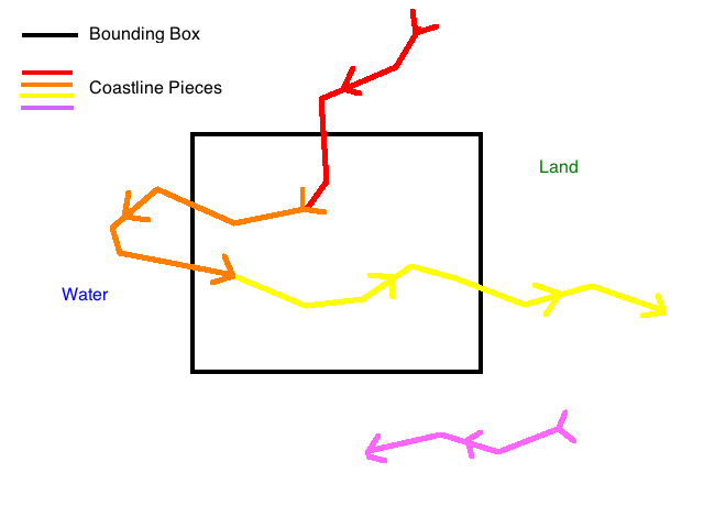
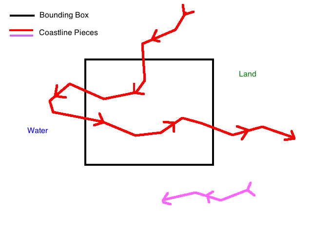
I ran into all of these issues during my time working on this project and I’ll address each of them here. The first step is to merge the various pieces of coastline returned by an OSM API query, which is not that difficult to figure out. As I mentioned before, you can assume that any connected pieces of coastline share a start/end point with each other; so if you have a piece starting at point A and ending at B, one from C to D, and another from B to C, you can connect the first to the last and the last to the second and get one coastline from A to D. If your query also includes another unconnected piece, say X to Y, treat it as separate. More than likely, it is the same coastline that goes “off screen” (out of your bounding box) for a while and then comes back, for example with a very narrow bay. The algorithm I’m going to outline can handle multiple separate coastlines, so you only need to join the ones that share endpoints.
It is probably worth putting a disclaimer here that I am not a mathematician and there is probably a better way to do this. I did do some cursory research, but I enjoy solving problems like this, especially in coordinate geometry; so when I didn’t find any obvious solutions I went about creating my own. To restate the problem more formally, you have a bounding box and one or more paths that may or may not pass through it. If you’ve joined the coastline pieces properly, you should be able to assume that none of the paths start or end inside the box; they either pass through it or they don’t. The goal is to form the correct closed polygons out of these paths and the bounding box. The key constraint that makes this possible is that the points that comprise coastline paths are by convention specified in clockwise order, which means that the water is always on the right-hand side of the path and land on the left.
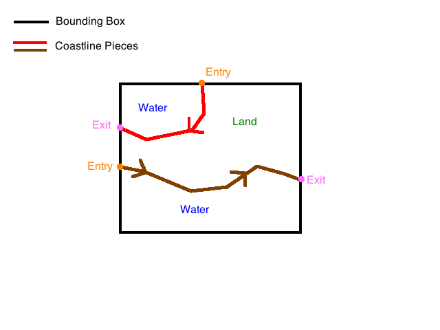
The first step of this algorithm is to clip all points in the coastline paths that fall outside the bounding box and create new points on the boundary of the box where these paths enter and exit. Aside from removing extraneous points, this will completely remove any coastlines that don’t pass through the box at all. It will also break any contiguous coastline that leaves the box and re-enters it later into two or more separate paths; this is perfectly okay. The entry and exit points created by this process are also required for creating the resulting polygons, as we will see shortly.
function clip(coastlines, box)
  clipped_coastlines = [ ]
  current_clipped_coastline = [ ]
  previous_point = nil

  for path in coastlines
    for point in path
      if nil_or_outside_box?(previous_point) and outside_box?(point)
        entrance_point, exit_point = intersection_points(box, line_segment(previous_point, point))
        clipped_coastlines << [entrance_point, exit_point]

      elsif nil_or_outside_box?(previous_point) and inside_box?(point)
        entrance_point = intersection_point(box, line_segment(previous_point, point))
        current_clipped_coastline = [entrance_point]

      elsif inside_box?(previous_point) and outside_box?(point)
        exit_point = intersection_point(box, line_segment(previous_point, point))
        current_clipped_coastline << exit_point
        clipped_coastlines << current_clipped_coastline

      if inside_box?(point)
        current_clipped_coastline << point

      previous_point = point
      return clipped_coastlines
I’m not going to provide full implementation details here. The functions for determining whether a point lies inside the box and computing where a line segment intersects a box can be imported from a library or implemented using basic linear equations. One thing I think is worth mentioning is that you should treat points on the boundary/corners of the bounding box as “outside” the box during all calculations. This avoids a lot of headaches; for example, the above algorithm assumes that any line comprised of two points outside the box will intersect it at either 0 or 2 points. Considering the corner points of the box to be “inside” would result in an additional scenario where it only intersects 1 point (a corner); thus it is best to just treat it as a miss instead.
We are now left with a set of paths whose start and end points lie on the boundary of the box and all other points are contained within it. We can safely assume a few things about these paths given the nature of coastlines: first, that they don’t intersect with each other, and secondly, that points along the boundary of the box will alternate between end and start (exit and entry) nodes of the various paths. This is important for the second part of the algorithm, in which we will move clockwise along the edges of the bounding box, creating polygons from the paths by adding corner points when necessary to close them.
function close(paths, box)
  finished_polygons = []
  current_path = paths.first
  current_polygon = [current_path]
  current_side = current_path.points.last.side
  first_side = true

  do
    next_path = find_next_path_on_side(paths, current_path, current_side, box, first_side)

    if next_path and next_path == current_polygon.first
      paths.delete(current_polygon)
      finished_polygons << join_paths(current_polygon)
      current_path = paths.first
      current_polygon = [current_path]
      current_side = current_path.points.last.side
      first_side = true

    elsif next_path
      current_polygon << next_path
      current_path = next_path
      current_side = current_path.points.last.side
      first_side = true

    else
      current_polygon << create_path( box.get_corner_point_for_side(current_side) )
      current_side = box.next_clockwise_side(current_side)
      first_side = false

  while paths.not_empty?

  return finished_polygons
Let me explain a few details as there is a lot going on here. For one, I am assuming that the start and end points of each path, which were computed by the previous function as the intersection points between the path and the bounding box, were annotated in some way to remember what “side” they were on. By this I mean which side of the bounding box: left, top, right, or bottom. Determining this is a natural byproduct of computing the intersection points if you are not using a library, as you will need to check for collisions with each side of the box individually. In addition to these annotations there is this notion of moving “clockwise” around the sides of the box, which as you would expect is the same as on a circle; if you started from the left side, for example, the clockwise order of the sides would be the same as I listed them previously.
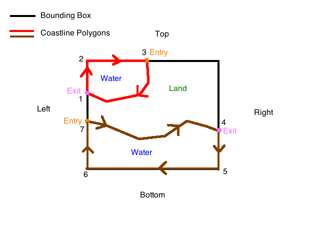
There is also the notion of “clockwise order” for points lying on the same side. Whether or not a point is clockwise to another point depends on which side they are on. If they’re on the left side, points [A,B] are clockwise if A.y < B.y; the reverse is true on the right. If they are on the top side, they are clockwise if A.x < B.x, and so on (this is of course in lat/lon space). The “corner point” for a given side is the most clockwise point that lies on that side of the box; for example, the left’s corner point would be the top-left point, the top’s would be the top-right, and so on. With that in mind, the next_clockwise_side and get_corner_point_for_side are trivial to implement. find_next_path_on_side is a little trickier so I’ll include an outline here.
function find_next_path_on_side(paths, current_path, current_side, box, first_side)
  same_side_paths = []

  for path in paths
    if path.points.first.side == current_side
      if not first_side or clockwise?(current_path.points.last, path.points.first)
        same_side_paths << path

  return sort_by_clockwise(same_side_paths).first
Going back to the “close” function, the algorithm takes the first path and starts on the side of the box where the path’s last (exit) point lies (indicated by its previous annotation). That path is added to the current polygon we are constructing. We then find the next path whose first (entry) point lies on the same side and is closest clockwise (the first_side flag is used here so that we can distinguish between when we are starting out and when we’ve wrapped back around). If this next path exists, we add it to the current polygon and continue our search in the same fashion from the side that this latest path’s last point lies on. If such a path does not exist, we add the corner point of the side we are currently on to the current polygon and move on to the next clockwise side, again attempting to find a path with an entry point on the current side. During this search if we encounter a path and we have seen that path before, we close the current polygon. We then remove the paths in the current polygon from the original list, join them together, and start a new polygon with the first remaining path. If there are no more remaining paths, we are done.
The polygons created with this algorithm should accurately represent where the ocean is present within your bounding box and can now be added to the SVG output in the same way you would render a lake or other closed body of water. This is probably a good time to note that some lakes are large enough where rather than return the entire lake, OSM will return a path segment similar to coastlines. You can easily check for this by verifying that the start and end point of the lake are not the same point. If this is the case, you can add the lake path to the coastline algorithm and get the same result. It is also worth mentioning again that islands are a special type of closed coastline that should be checked for and rendered as a closed green polygon rather than run through the above algorithm.
Ocean Detection
The last major problem I ran into with regard to oceans was detecting whether my bounding box was inside the ocean or on land. This is easy with the presence of a coastline or an island, but if neither are returned in your bbox query the API provides no way of knowing whether you are in the middle of the ocean or the middle of the desert. I tried various heuristics as our game really only needed to be accurate for some number of tiles off the coast, but these turned out to be unreliable.
This appears to be a problem more than one person has encountered and thus there is a somewhat standard solution within the OSM community. This involves using a small subset of the global OSM data containing only the world’s coastlines at the lowest acceptable resolution to first determine whether you are in the ocean or not. This subset is stored in a shapefile, a compact binary format that contains hundreds of thousands of polygons representing the Earth’s land area. You compare the box or a point within it to each polygon and if it is contained within one of them, the box is encompassed by land. If not, you are in the ocean. These files (shoreline_300 for super-low resolution or processed_p for higher resolution) and be downloaded from the OSM wiki on the “coastlines” page.
This brute force comparison is obviously horribly inefficient, especially for a data set this size. It can be sped up considerably by comparing to the bounding box of each polygon first (included in the shapefile) and then only comparing to the polygon itself if the tile’s bounding box is within the polygon’s. This is still slow, however. The next step would be to arrange the polygons’ bounding boxes in a binary tree index of some sort for faster searching, optimize how the file is loaded and kept into memory, etc. Implementing all of this yourself is completely pointless as there is already perfectly good software out there that does this for you: relational databases. Namely, relational databases with geospatial extensions. Postgres (PostGIS) is the most popular and feature-rich, but since we were already using MySQL I decided to go with that.
MySQL has had geospatial support for some time, but apparently it has been sorely lacking in features up until version 5.6, which is still relatively recent in the world of MySQL; as of this writing it is not the version you will find in most package managers, so be warned. The spatial extensions allow you to natively store, index on, and query columns containing points, polygons, and other geometry extremely fast. We simply need to create a table with one column of type “geometry”, create a spatial index on that column for fast querying, and import the shapefile into the table. A row is created for each polygon in the file. Note that spatial indexes are only supported on myISAM tables and the geometry column cannot be null.
CREATE TABLE `land_polys` (
  `id` int(11) NOT NULL AUTO_INCREMENT,
  `poly` geometry NOT NULL,
  PRIMARY KEY (`id`),
  SPATIAL KEY `poly` (`poly`)
) ENGINE=MyISAM
If you’re comfortable working with binary files you can parse the shapefile yourself and insert the polygons into the database; the shapefile format is documented on Wikipedia. If you’re using Ruby there is a gem called RGeo with a shapefile reader extension that you can use to parse the file instead. Note that you must use the GeomFromText MySQL function to convert the polygon from it’s Well Known Text Format (WKT; just call to_s in RGeo) to MySQL’s native format. Consult the MySQL documentation for more details.
Once you’ve imported the coastline data into the database, you can query it from your application to determine whether or not the current tile is on land or in the sea. This is done using the ST_Contains query function, which will search a given geometry column for all rows that contain the passed-in geometry. I just used the midpoint of the tile since anything else is probably overkill. If the query generates a non-empty response, there was at least one polygon that contained the passed-in point and thus your tile is over land.
SELECT * FROM land_polys WHERE ST_Contains( poly, GeomFromText( 'POINT( x y )' ) )
Using this database, combined with checking for the presence of coastlines and islands, should allow you to accurately determine what the “background color” of your tile should be (land or water). This is the last piece of the puzzle needed to implement a reasonably fast and accurate vector map tile service that can display roads and bodies of water, and can be easily extended to display other geographic elements. In fact after comparing the output of my service with Cloudmade’s, I’m pretty confident they used the same technique for their now-deprecated vector API. An added bonus of this particular approach is that even if MapQuest decides to pull the plug on their API endpoint, we can simply switch to another OSM provider or even set up our own as a last resort.
Deployment
Of course, this service is of no use to anyone unless it is deployed somewhere and is scalable enough to be used by our game. This is still a work in progress, but I’d like to share what I’ve discovered so far; just be aware that this section is subject to change.
I implemented my vector tile service in Ruby as a Sinatra app, as I felt Rails was too heavyweight for an API with one or two endpoints and no models. I had somewhat of an idea going into the deployment phase what to expect performance-wise from testing on my local machine. The service is essentially bound to the OSM API call, which can take anywhere from a quarter to a full second depending on the zoom level and how much data is returned. There is not really anything we can do about this on a per-request basis except cache aggressively, which I will get into momentarily. Fortunately, our game does not require millisecond response times; waiting one second for the map to load is perfectly acceptable, as it is in most mapping applications. Map tiles do, however, lend themselves well to parallelization. There is no reason to wait for a tile to be returned before requesting another one, and indeed this is what our game does in order to minimize load time.
Caching is a no-brainer in situations like these where the same content is being requested by multiple clients and said content rarely changes. There are a variety of ways to accomplish this; we opted for a simple solution for the time being, writing out each response to the filesystem based on tile size, x, y, and zoom. We then configured Nginx to bypass our app and simply serve the static file if one was present for that tile, which is extremely fast. Given the number of tiles in the world, precaching was not really an option, nor was it desirable; the vast majority of tiles will never be requested anyway, whereas a small subset (such as those in major cities) will be requested very frequently and quickly cached. In fact, we speculate that after some period of time the overwhelming majority of requests to the tile server will be served out of the cache.
Of course, our deployment still has to survive the initial onslaught of clients while the cache warms up, each with multiple parallel connections. I deployed our service to a medium AWS instance, with the Sinatra app being served by 8-16 Unicorn workers running behind Nginx. I pointed my iOS simulator running our game to it and monitored the performance, which turned out to be very disappointing. Not only was it noticeably slow loading tiles on the client, the server CPU usage spiked to 100% during this time from just one consumer. Since we are hovering around 1,000 DAU at this time and growing, this was not going to cut it.
It occurred to me relatively quickly that each Unicorn worker was blocking for up to a full second during the OSM API call and during that time could not handle any other requests as Ruby MRI is not natively threaded. Thus the number of concurrent requests, with only 16 workers, was extremely limited. As someone who is not intimately familiar with systems programming, I was also unsure how intelligent Linux is about context switching these worker processes; was it possible it was allowing them to spin the CPU instead of deprioritizing them during these HTTP calls? I wasn’t sure. The obvious first solution is to fire up more workers, but even though this is a lightweight app each process needs its own copy of the environment and this takes up a lot of memory; also, switching between processes is expensive. It seemed like a waste to throw more computing resources at the problem when they were obviously being used so inefficiently.
The second solution I came across was to use a threaded web server. This way, only one copy of the environment would need to be loaded, and context-switching between threads is much faster and (presumably) more intelligent. The problem is that Ruby, from what I understand, does not support true multithreading. JRuby however, which runs on the JVM and taps into its threading capabilities, does. I will spare you the details, suffice it to say that I’ve used JRuby in the past at Shareaholic and due to compatibility issues it can be quite the headache to get up and running. Additionally, it seems to require a bit more of an upfront outlay of hardware resources; after setting it up using several different application containers on the aforementioned medium AWS instance, the resulting performance was considerably worse than even before. This could have been the result of JIT firing up, or it may have been a lack of proper configuration on my part. This is one of the other pitfalls of JRuby; you inherit all the fun of dealing with Java application containers.
I quickly abandoned this approach as I was much more intrigued with a third type of solution: asynchronous web servers. If you’re familiar with Node.js then you’ve heard of this concept before. Rather than spawn a separate process or thread per request, these servers handle everything in a single event loop. In order to accomplish this, the server and the application it is hosting need to strictly utilize non-blocking (asynchronous) IO. All network requests, calls to the database and filesystem, etc must return immediately, otherwise they will block the main event loop and the whole server will grind to a halt. When they are done with their business, an event is triggered and a callback is processed. This allows the server to handle many requests at the same time.
There are several asynchronous web servers for Ruby applications, most built on top of an event processing library called EventMachine that provides asynchronous IO. I chose to use Thin, which is an evolution of the synchronous and formerly popular Mongrel server. Thin has actually been around for a while, but it does not enforce using non-blocking IO and so if you’re not careful you can end up with just another synchronous Mongrel deployment, which is apparently a common problem. I also used the em-synchrony gem, which patches the EventMachine libraries to take advantage of fibers, and the sinatra-synchrony gem, which configures Sinatra to put each request in a fiber so that it can take advantage of em-synchrony and Thin. A newer alternative to Thin is Goliath, which uses em-synchrony and fibers by default and provides more of an integrated, pre-configured package.
Note that fibers and the em-synchrony library remove the need to write callbacks; you simply write your code as if it were blocking and the fibers will transfer control back at the appropriate time. Thus, very few changes were required to the code itself to convert to asynchronous IO. The HTTP call to the OSM API was my primary concern and the reason for this approach in the first place. I was previously using Ruby’s net/http, but switched over to using Faraday, which supports multiple backends including em-synchrony. Other than that, no other changes were necessary. em-synchrony also provides an asynchronous wrapper around the mysql2 gem, which I took advantage of as well. However, because the database is located on the same machine as the app and the one query I need to run takes less than 10 ms, it is not strictly necessary to make the call non-blocking. Similarly, I did not opt to make the caching writes to the filesystem asynchronous, though if it becomes an issue I will do that as well.
Switching to an asynchronous deployment increased performance considerably, though the CPU still sustains a higher load than I would like. As I said, this is a work in progress. We haven’t yet had to go live with it, but it is possible that day will come soon. There are still a few features we would like to add as well, such as returning the names of towns and neighborhoods. This requires another call to the OSM API (this time for nodes) and degrades performance considerably. I’m looking into a solution similar to ocean detection, where a small data subset is imported into a database for easy lookup (update: inserted MaxMind city file into database to do spatial search similar to oceans). Whether or not this service sees the light of day, it has been an extremely interesting and challenging project, and I’ve enjoyed working on and writing about it.